In this exemplary project, Cell line Expression atlas Gene expression data is used to create a state-of-the-art Machine learning model to classify leukemia and separate it from the other types of Cancer.

You may find the code and additional data on the main GitHub repository : https://github.com/DarkoMedin/cancerclassifier_L

The dataset contains of 50 000 genes and over 1000 classes of cancer. The goal is to create a classification model to predict leukemia as a class and separate it from other cancers.

Here is the link to the dataset and I advise you to read more about different aspects of the data on this link.

https://www.ebi.ac.uk/gxa/experiments/E-MTAB-2770/Downloads

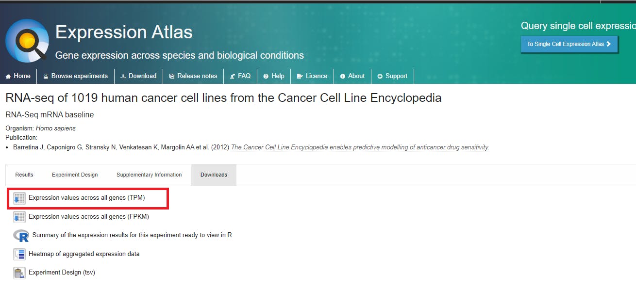
The downloaded file, E-MTAB-2770-query-results.tpms is the main dataset for the exemplar project. The dataset is associated with the reference publication, Barretina J, Caponigro G, Stransky N, Venkatesan K, Margolin AA et al. (2012) The Cancer Cell Line Encyclopedia enables predictive modeling of anticancer drug sensitivity.

Now open the dataset in Python. For this tutorial, I will be using https://colab.research.google.com/ (Google Colab)

First, make sure you have loaded the libraries (and previously installed them).

import numpy as np
import pandas  as pd
import seaborn as sns
import matplotlib.pyplot as plt
from sklearn.model_selection import train_test_split
from lightgbm import LGBMClassifier
from sklearn.preprocessing import LabelEncoder 
import matplotlib.pyplot as plt
from sklearn.metrics import accuracy_score
from sklearn.metrics import confusion_matrix, ConfusionMatrixDisplay
from sklearn.metrics import accuracy_score
from sklearn.utils import shuffle

As you can see the main libraries for the project are, pandas, numpy, seaborn, lightgbm, sklearn and matplotlib. I will use the left pane on the google colab doc to upload the dataset E-MTAB-2770-query-results.tpms in the workspace and I can load it directly from there and examine it using the following code:

df=pd.read_csv(r'E-MTAB-2770-query-results.tpms.tsv',
             sep="\t", comment='#')
df=df.loc[:,~df.columns.str.contains('normal', case=False)]
df 

#If you are using your local file stored on your PC add the path before filename

The second line of the code is used to remove the 8 normal cell lines. Remember, the goal is to classify leukemia vs other cancers and normal cell lines don't beling to any of the classes and will be removed to avoid the wrong classification of those 8 samples.

This is the produced output

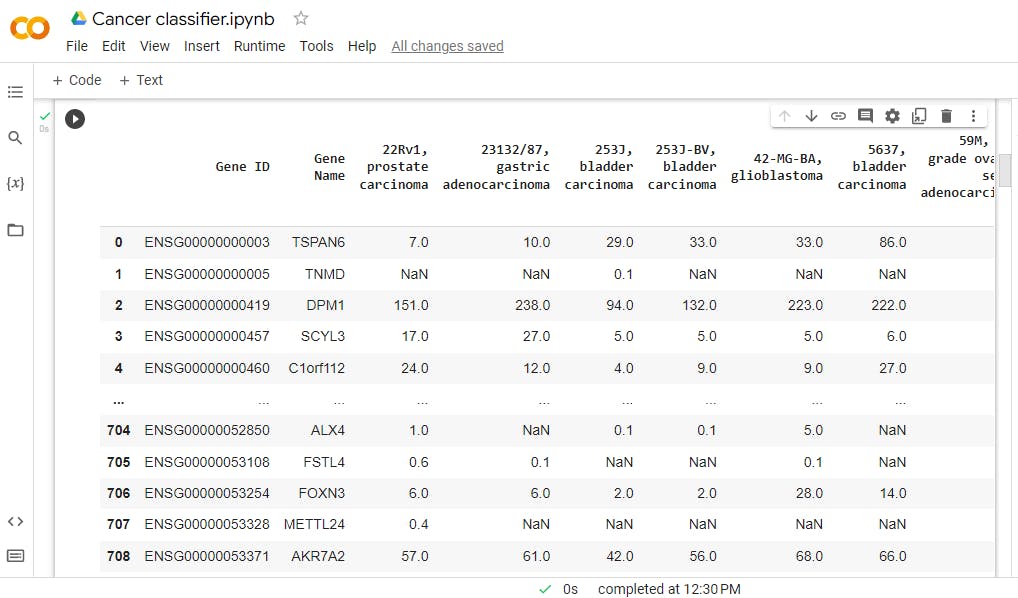
You may notice the value of gene expression and these are tpms or a unit called transcripts per million.

Here is the next block of code:

One of the most important variables in our data is the target variable, the one we are trying to predict. In this dataset there are over 50 000 predictor genes and just 1 target variable. This tells you about the importance of that 1 target variable, so one must be very accurate with it to produce the wanted result.

Let's define the target variable as a list. Since the column names contain the target cancer types, we can use those names and create a list of them.

#Define the targets for prediction (cancer samples)
target=list(df.columns[2:])

The next step is to create the function engineer the labels the way we want them to be classified. In this case, the labels are to be leukemia ( if the label contains the word leukemia) and other cancers ( if the label does not contain the word leukemia)

def eng_labels(x):
   labs=[]
   for s in x:
         if 'leukemia' in s:
             labs.append('leukemia')
         else: 
             labs.append('other cancers')
   return(labs)

Voila, the function eng_labels is created. It can now be used to separate leukemia from other cancers in the target variable.

labs=eng_labels(target)
labs=['Gene']+labs
labs=pd.Series(labs)

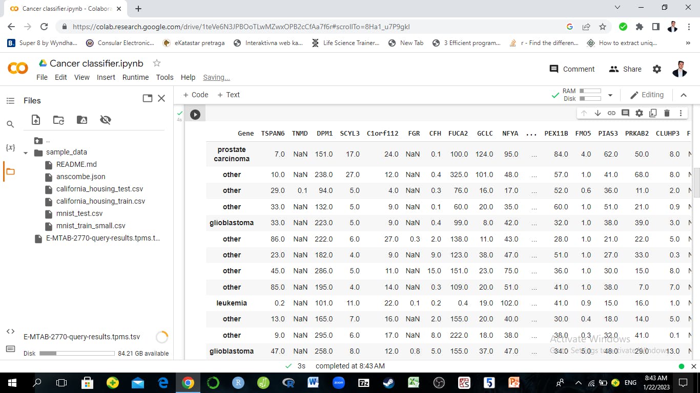
Using the eng_labels function the labs variable is created and it contains only leukemia and other cancer targets. But to prepare the data for training the classification model, there is still some work to do. The dataset contains a column 1 we don't need and we will need to transpose the dataset so the genes are the columns. Why is this needed? The standard principle of many Classifiers is to read columns as variables and rows as samples. The goal is to have the genes as predictors and the target variable as a predicted variable. The genes (and gene names on top) will need to be columns and not rows.

So transpose() function from pandas will do the work and convert the data in a format with variables as genes and rows as samples.

data=df.iloc[:,1:]   
data.columns=labs
data=data.transpose()
data.columns=data.loc['Gene',:]
data=data.iloc[1:,:]
pd.set_option('display.max_rows', 20)
pd.set_option('display.max_columns', 20)
data.head(20)

The output:

Now let's do some EDA on the individual genes. RNA seq data generally has negative binomial distribution and even if it's normalized as in this case (tpm normalization), the data should be skewed towards the right. This means most of the data and the data peak will be on the left side of the distribution and the long tail will be on the right.

Lets check this for a couple of genes...

sns.histplot(data['SCYL3'], kde=True)

The SCYL3 gene has the distribution just as described, Most of the gene expression values are between 0 and 20 tpm while a very small fraction of genes is between 20 and 40 tpm.

The histogram for the DPM1 gene...

sns.histplot(data['DPM1'], kde=True)

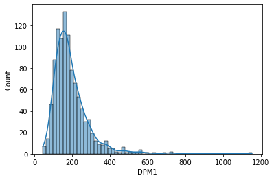
DPM1 gene has a similar shape to the distribution, skewed toward right with the peak on the left side, but the values of gene expression are much higher with most of the values between 0 and 400 tpm. You can see that values of gene expression may vary a lot, but their overall shape of the distribution is similar and it originates from the negative binomial distribution which is typical for RNA seq data.

And another gene distribution...

sns.histplot(data['MSMO1'], kde=True)

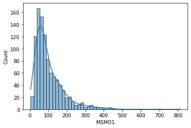
MSMO1 gene has a similar shape and distribution to the previous one, DPM1.

Now a bit of data engineering...

To prepare the data for Machine Learning, some more things need to be done:

1. Perform the label encoding (labels represent the classes). I want them to be numbered, so 0 and 1 can represent the 'leukemia' and 'other cancer' classes. For this, I will need the label encoder from sklearn.

2. Impute the missing values, for this, I will need KNN imputer from sklearn.

The code:

data_x=data                       
data_x=np.array(data_x)
le = LabelEncoder()
le.fit(data.index)
data_y=le.transform(data.index) 
data_y=pd.Series(data_y)

The objects are created now as data_x, which contains the predictor genes and data_y which contains the labels as 0s and 1s ('leukemia' and 'other cancer classes')

xtrain, xtest, ytrain, ytest = train_test_split(
 data_x, data_y, test_size=0.33, random_state=87)


#This is needed to facilitate the training process
xtrain=np.array(xtrain, dtype=np.float32)
ytrain=np.array(ytrain, dtype=np.float32)


xtrain, ytrain=shuffle(xtrain, ytrain)
xtest, ytest=shuffle(xtest, ytest)

Now that we have confirmed that the data is heavily skewed and preprocessed the data, a choice of classifier algorithm can be made. In this case, it's the best choice to use a tree-based method, which should perform well on a large number of variables with skewed normalized data. Since there is a lot of data, and i want high accuracy, a method that can be trained in a lot of epochs but still quickly enough is needed.

A method called LGBM or light gradient-boosting machine is a method that can produce high accuracy with skewed data, and a lot of variables and can do this while being trained quickly in a lot of epochs. Ideal combination!

LGBM has a lot of parameters and these parameters are something I created using a lot of experimentation and tuning. You may also experiment with a different combination. Here is my combination of parameters and I will store them in a python dictionary.

p={ 'boosting':'dart', 'learning_rate':0.01, 'objective':'binary', 'max_depth':6
   , 'num_leaves':102, 'min_data_in_leaf':35, 'bagging_fraction':1,'device_type':'cpu',
   'feature_fraction':1, 'verbose':0, 'bagging_freq':7, 'extra_trees':'true','cegb_tradeoff':5,
  'max_bin':100, 'min_data_in_bin':2,'n_estimators':15750}

Keep the learning rate low ( in this case 0.01) and n_estimators, which is actually a number of trees as quite high (in this case 15750).

Notice that 'dart' booster is used. The dart method is one of the best options for gene expression data. I will keep the max depth at 6. Going over 6 can cause serious overfitting.

Now when the parameters are set, I can use the **p statement and fit() function to train the LGBMClassifier model.

lgbmodel=LGBMClassifier(**p).fit(xtrain, ytrain)

It might take a while to finish the training. Depending on your CPU or GPU used, it might take anywhere from 30 seconds to 10 minutes. This is fast as using other methods like XGBoost or Deep Learning, the training could take hours or even days. After the training is finished the model can be used to predict the new values. The new values are those to which the model was not exposed during the training and are a good test for the accuracy of the model.

Predicting new values and accuracy assessment.

predictions = lgbmodel.predict(xtest)
rpreds = [round(i) for i in predictions]
accuracy = accuracy_score(ytest, rpreds)
accuracy

0.9880239520958084

The overall accuracy of 97.92% includes both leukemia and other cancer predictions. What we also want to know is how accurate the model is at predicting the leukemia cancer. To be able to understand this better, let's create the confusion matrix which will facilitate the interpretation.

Notice how I used round to create rpreds because most machine learning models output probability for classes and not classes, so we need to use the round() function to convert them to the most probable predicted classes.

Output:

predictions = lgbmodel.predict(xtest)
cm = confusion_matrix(ytest, predictions)
disp = ConfusionMatrixDisplay(confusion_matrix=cm)
disp.plot()
plt.show()

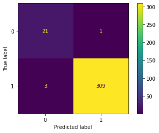
As you can see the labels 0 represents the leukemia and label 1 are other cancers. The dataset is heavily unbalanced towards other cancers which is logical as leukemia is just one of many types of cancers. But even with that imbalance, the classifier was quite accurate for leukemia. It predicted 21 out of 25 leukemia cases in the test set correctly and that would be 84% accuracy in predicting leukemia classes, which is still impressive on a dataset of around 1000 samples and a real partition of the test data.

importances=lgbmodel.feature_importances_
importances=pd.Series(importances)
importances.index=data.columns
importances= importances.sort_values(ascending=False)
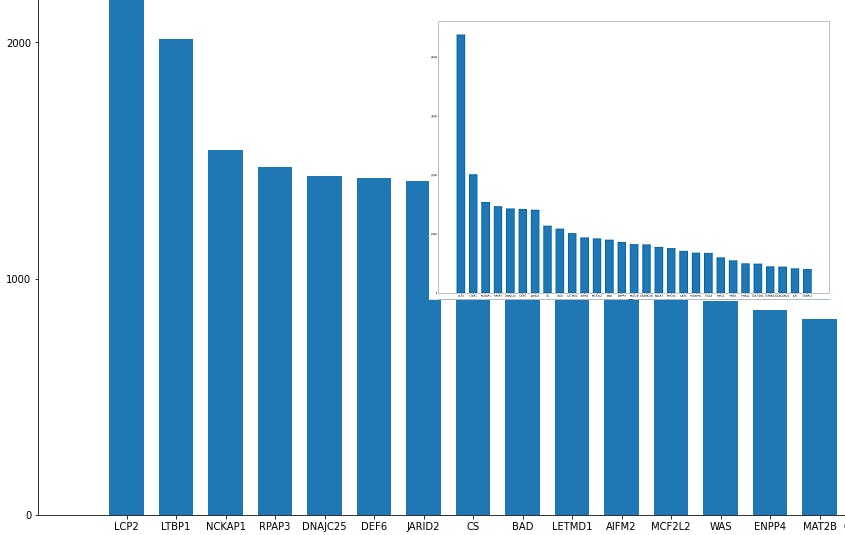
importances[0:29].to_csv(r'important_genes.csv', sep='\t', header='true')

The file important_genes.csv now contains the 30 most important genes for this classifier.

plt.figure(figsize=(28,20))
plt.bar(importances[0:29].index, importances[0:29], width=0.7, bottom=None, align='center', data=None)

Thank you for reading!

Created by Darko Medin

All information in this exemplar project is for research and educational purposes and should not be considered as any form of professional medical aspects.

Software used:

https://www.python.org/

https://pandas.pydata.org/

https://numpy.org/

https://scikit-learn.org/stable/

https://lightgbm.readthedocs.io/en/v3.3.2/

https://seaborn.pydata.org/

https://matplotlib.org/